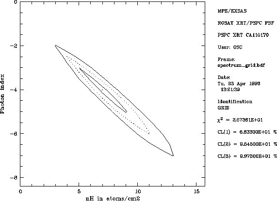
Figure 6.3: Contour plot of
Here we start with an observed spectrum testdata1:spectrum.tbl of our source. We assume that this spectrum is already corrected by using the correction mode of the projection package (see last example and chapter 4) and begin with setting the context to exsas.
Midas 001> set/context exsasFirst we bin the detector response according to the observed spectrum. We relate the binned detector response matrix to the name of the observed spectrum spectrum_drm instead of using the default.
Midas 002> bin/detector testdata1:spectrum ? spectrum_drm
 Create binned detector response matrix spectrum_drm.
Accordingly we create the parameter file spectrum_grid.par necessary to produce the
Midas 003> CREATE/PARFIL fit spectrum_grid ? ? ? expert
!
! --- general key words ---
!
FIT                                     ! alternative: COMPARE, CALCULATE
FOLD                                    ! folding with detector response
INPUT_FILE      testdata1:spectrum      ! observed X-ray spectrum
OUTPUT_FILE     spectrum_grid           ! 2-D grid of chi-square values
CORRECTION_FILE exsas_cal:effarea_pspcc ! corrected effective area
RESPONSE_FILE   spectrum_drm            ! binned detector response matrix
!
! --- power law model, parameters, and red shift ---
!
MODEL        gamm(1)*powl(2,3,4)        ! galactic absorption * power law
PARAMETER 1  0.0  15.0   1.0      grid  ! nH, units of 10^21 atoms/cm^2
PARAMETER 2  1.E-2 1.E-7 1.E+5 0. free  ! flux amplitude at E0
PARAMETER 3  -8.0  0.0   0.5      grid  ! photon index gamma
PARAMETER 4  1.0                        ! reference energy E0 in keV
REDSHIFT     0.0                        ! red shift z

Figure 6.3:
Contour plot of ![]() as a function of the galactic
column density
as a function of the galactic
column density ![]() and the photon index
and the photon index ![]() for
three confidence levels of 68.3%, 95.4%, and 99.7%
for
three confidence levels of 68.3%, 95.4%, and 99.7%
Now we run the command MODEL/SPECTRUM to search for
a ![]() grid. Since the program runs
grid. Since the program runs ![]() single fits it takes a while to output the results
in the bulk data frame spectrum_grid.bdf.
single fits it takes a while to output the results
in the bulk data frame spectrum_grid.bdf.
Midas 004> model/spectrum spectrum_gridWe create a graphic window to make a contour plot of confidence levels by using constant
Midas 005> create/graph
Midas 006> set/graphic pmode=1 fonts=1 frame=square
Midas 007> plot/chi2_contour spectrum_grid 3 ? xlab="nH in atoms/cm2"
ylab="Photon index"
Midas 008> copy/graphic LASER