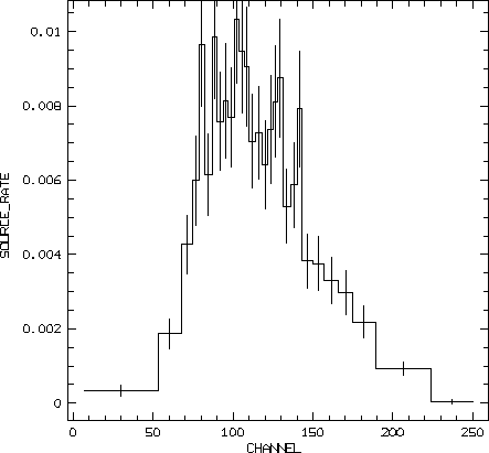
Figure 6.1: Binned spectrum taken by the position sensitive proportional counter of the ROSAT X-ray telescope
Starting from a given photon event file testdata1:events.tbl, a raw spectrum is binned from all events coming from a circle around the selected source as well as from a surrounding background (table raw_spectrum). Here we set the data projection in correction mode (for details see chapter 4). After that a background subtracted count rate spectrum of the source is prepared (table spectrum) and fitted with a power law model. The fit result is output to table spectrum_o. A standard plot of the fitted spectrum closes this session.
If EXSAS is not automatically running, which depends on the current system setup, we enter EXSAS in the MIDAS environment by setting its context to EXSAS:
Midas 001> set/context exsasFor correcting the data we have to access the effective area of the actual XRT PSPC detector ``C'' located in the EXSAS calibration area. Here the dead time correction is not applied.
Midas 002> set/projection correct=exsas_cal:effarea_pspccFrom spatial analysis we know the approximate position of a point source in sky pixels: 503,-4504. We select photons from a circle and a ring around the source from file testdata1:events, bin their pulse height amplitude, and output the raw spectra into table raw_spectrum.
Midas 003> select/ring [503,-4504,500][503,-4504,600,1900]
           bin ampl 1,8,250 *testdata1:events *raw_spectrum

Figure 6.1:
Binned spectrum taken by the position sensitive proportional
counter of the ROSAT X-ray telescope
To get a count rate spectrum of our source and its background (output file spectrum), which is the input of the fitting procedure, we run prepare/spectrum. We use the option sigma to bin the spectrum in such a kind that each bin at least contains a count rate with a signal to noise ratio of 5.
Midas 004> prepare/spectrum raw_spectrum spectrum ? 5We create a graphic window, choose a proper graphic mode and plot the count rate spectrum of the source (see Figure 6.1).
Midas 005> create/graph
Midas 006> set/graphic pmode=0 frame=square
Midas 007> plot/spectrum spectrum s y
Now everything is ready to start the fit, except, that we have to define a model. To fit a simple power law model to the data it is enough to use a four letter acronym powl (preserved name) instead of the name of a parameter file. In this case a special parameter file is copied to the working area under the name spectrum_powl.par. Since we have chosen the correction mode for the data projection the correction vector table has to be replaced by the corresponding effective area table exsas_cal:effarea_pspcc, which has to be the same as specified in the set/projection command. By default response matrix exsas_cal:drmpspc_ao1 is chosen, since this was a very early observation.
Figure 6.2:
Power law fit to an observed X-ray spectrum (PSPC)
with residuals and the corresponding unfolded
model-dependent monochromatic photon flux.
Midas 008> fit/spectrum powl spectrum ? exsas_cal:effarea_pspcc
 descriptor OBS_CLOCK < 42907994.54  -->  AO-1 or earlier:
 using default response matrix exsas_cal:drmpspc_ao1.bdf
bin/detector spectrum exsas_cal:drmpspc_ao1 drmpspc_ao1
 Create binned detector response matrix drmpspc_ao1_b.
model/spectrum spectrum_powl.par spectrum spectrum_o
 exsas_cal:effarea_pspcc drmpspc_ao1_b
 ...
 ...
 ---------- Convergence ! ----------
 P* parameter, E* correlated error, D* uncorrelated error
 P1=  7.758     P2= 2.9158E-02 P3= -4.461
 E1=  2.924     E2= 7.6260E-03 E3=  3.508
 D1=  2.905     D2= 2.2378E-02 D3=  1.408
 Initialize table spectrum_o.tbl.
We plot the result of the fit and send a copy to laser printer LASER. This plot can be seen in Figure 6.2.
Midas 09>  plot/fit spectrum_o ? ? nice
Midas 010> copy/graph LASER