In this section some examples are given of how to create hardness ratio images, time series and color-color diagrams making specific reference to the ROSAT-PSPC case. The SASS standard hardness ratio definitions will be used (see Table 4.1).
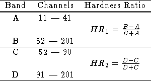
Table 4.1: Definition of standard hardness ratio for ROSAT-PSPC data
In order to correct images for vignetting and dead time projection has to be used in the correction mode SET/PROJECTION CORRECT (see section 4.3.4).
Midas 001> SET/PROJECTION CORRECT
Midas 002> SELECT AMPL [11,41][52,201][52,90][91,201] -
            BIN/IMAGE 30 in=events out=imagea,imageb,imagec,imaged
With the above projection pipeline four images named imagea.bdf, imageb.bdf, imagec.bdf and imaged.bdf are created in the energy bands A, B, C, and D.
The HR_1 and HR_2 images are created with the following two MIDAS commands:
Midas 002> COMPUTE/IMAGE hr1 = (imageb-imagea)/(imageb+imagea)
Midas 003> COMPUTE/IMAGE hr2 = (imaged-imagec)/(imaged+imagec)
In the production of images containing energy information it is anyway suggested to make use of the ENERGY option in the data projection. The images created when this mode is on are much richer in information than any hardness ratio image. One pixel value of an ``energy'' image is the average of the calibrated pulse height channel (table column AMPL) of all the photons which contributed to that pixel (the calibrated pulse height channel is a quantity related roughly linearly to the energy of the photon).
The production of an ``energy'' image is much simpler and faster than the production of hardness ratio ones:
Midas 004> SET/PROJECTION ENERGY
Midas 005> BIN/IMAGE 30 inp=events outp=imagecol
In order to display such images, the usage of the Look Up Table energy is suggested.
The procedure for the creation of time series of hardness ratio is quite similar to the production of hardness ratio images. With the following pipeline four light curves with time bin of 10 sec, one for each of the defined energy bands, are created and written to the table rates.tbl at the columns labeled BAND1, BAND2, BAND3 and BAND4:
Midas 006> SELECT/RING cursor SELECT AMPL [11,41][52,201][52,90][91,201]-
           BIN TIME 10 ID=BAND *events *rates
After this, the hardness ratio can be computed via the MIDAS commands
Midas 007> COMPUTE/TABLE rates :HR1 = (:BAND2-:BAND1)/(:BAND2+:BAND1)
Midas 008> COMPUTE/TABLE rates :HR2 = (:BAND4-:BAND3)/(:BAND4+:BAND3)
This calculation is done without any error handling.
Finally, color-color diagrams might be easily produced by a sensible usage of the MIDAS commands SET/GRAPHIC and PLOT/TABLE applied to the data columns of the table rates.tbl.
In order to make things more accurately, the light curves should be corrected before the computation of hardness ratio. How to perform light curve correction is extensively described in sections 4.3.4 and 4.1.2. Otherwise, already corrected light curves can be created directly by setting Projection in correction mode via the SET/PROJECTION command (only for PSPC data, see section 4.3.4 for details).