Known-in-advance Period Detection

   

In this example, let's assume the photons corresponding to the desired source have already been extracted (via PROJECTION) from the original photon event table, and are contained in the PET sourx.tbl. Of course the column :TIME must be present. The source coordinates are .

The table must be sorted in time before using any timing command (they would not work otherwise): this is done with the command

SORT/TABLE sourx :TIME

  The first move will be to apply to the arrival times a correction to the barycenter of the solar system: in order to do this, the file containing the orbital information of the satellite must be used. In this example its name will be orbit_file.tbl. As a first step, a correction table corr.tbl must be created from the orbit file. The second step is to apply the barycentric correction to the photons.

CORRECT/ORBIT_DATA corr 5,40,35 -69,23,46 orbit_file
CORRECT/BARYCENTER sourx corr 5,40,35 -69,23,46

The correction on the arrival times is done in place, and the times are converted from Spacecraft Clock to Julian Day. The source coordinates have to be re-typed to check for consistency.

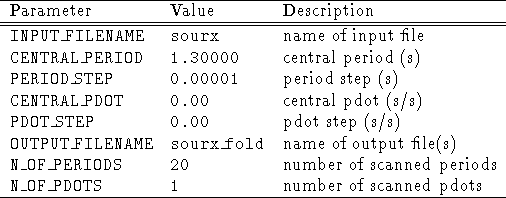
Now, the photon event table is ready for the analysis. Since we know (approximately) the period we expect from the source, we can use a period search based on the folding technique. To do so, a parameter file must be created first (see Table 7.1) by calling CREATE/PARFIL FOLD folding.par.

Note:Parameter files are all ASCII files. Each line should contain a parameter keyword (first column in the following tables) followed by the parameter value (second column). Additional comments (or whole comment lines) can be started with exclamation marks (!). The order of the parameters is not important, and parameters for which a default is present can be omitted.

  
Table 7.1: Example of a parameter file for period folding

With this parameter file a folding search will be performed on the sourx.tbl file, scanning 20 periods (with no period derivative), the central period and the step width are given. The statistical test used (default) is a . The light curve corresponding to the highest  will be stored in the table sourx_fold.tbl, and the  map as a function of period (it can be made two dimensional by stepping on period derivatives as well) will be stored in the MIDAS image sourx_fold.bdf. If the name of the parameter file is folding.par, the folding search can be run by typing

MAKE/FOLDING folding

To plot the resulting light curve (with errors) one can use the commands:

CREATE/GRAPH
PLOT/PULSE_PROFILE sourx_fold lstyle error_bar

where lstyle defines the line style used for the plot and error_bar defines if error bars are plottet or not (cf. Figure 7.1). The  curve as a function of period can be displayed with the MIDAS command PLOT/ROW sourx_fold.

  
Figure 7.1: Pulsar light curve generated using PLOT/PULSE_PROFILE