

Next: Extraction of Information
Up: Image Manipulations
Previous: Transformations
Both the imaging system and observing conditions will cause a
degradation of the resolution of the image. In principle it is
possible to reduce this smearing effect by deconvolving the frame with
the point spread function. The degree to which this can be done
depends on the actual sampling of the image. Basically, it is not
possible to retrieve information on features with frequencies higher
than the Nyquist frequency (see Equation 2.2). Several
different techniques are used depending on the data (see Wells 1980
for a general discussion of the methods).
Fourier transforms are often used since convolutions in the frequency
space become multiplications (see Section 2.3.3). Combining
Equation 2.1 and Equation 2.26 the
original image
 is obtained by division
![\begin{displaymath}{\cal I}(u,v) = {\cal O_F} [ F(j,k) \otimes P(j,k) + N(j,k)] / {\cal P}(u,v)
\end{displaymath}](img111.gif) |
(2.27) |
if the transformed PSF  is non-zero and the noise N is
insignificant. For data with low or medium signal-to-noise ratio
(i.e. S/N < 100), as for most optical observations, this technique
introduces artifacts in the deconvolved image. These effects can be
reduced by filtering the transforms with Wiener filters (Helstrom
1967, Horner 1970).
Another group of image restoration algorithms use iterative methods to
obtain a solution which is consistent with the data.
The maximum entropy method uses either the entropy :
 |
(2.28) |
in the optimizing procedure (Frieden 1972).
It tends to enhance sharp features but a solution may depend on the
initial guess and therefore not be unique.
A different scheme was introduced by Lucy (1974) who uses a correction
term based on the ratio between the image and the guess. A first
guess  must be specified (e.g. a constant) to start the
iteration. The first step in the iteration performs a convolution
with the PSF :
 |
(2.29) |
The second step computes a correction factor based on this frame and
the original image
 :
:
 |
(2.30) |
The procedure repeats these two steps until the corrections are
sufficiently small. After Equation 2.30 is computed
the iteration continues with Equation 2.29. This
scheme reaches a stable solution very quickly (i.e. 3-5 steps) and is
little affected by noise. This makes it very useful for low
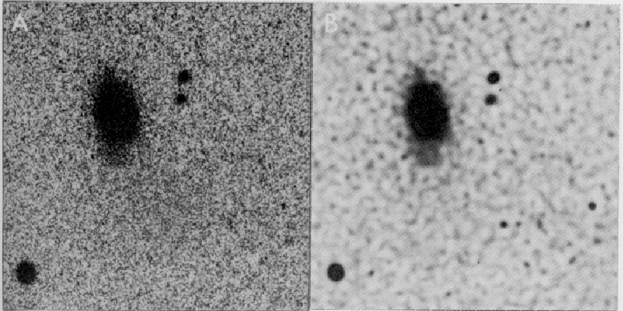
signal-to-noise data. A photographic picture of a galaxy is used to
illustrate this technique (see Figure 2.11). A fit
to the stellar image was used to define the PSF.
Figure 2.11:
Deconvolution a photographic image with the Lucy method:
(A) original and (B) restored image after 3 iterations.
 |


Next: Extraction of Information
Up: Image Manipulations
Previous: Transformations
Petra Nass
1999-06-15
![]() is obtained by division
is obtained by division
![]() must be specified (e.g. a constant) to start the
iteration. The first step in the iteration performs a convolution
with the PSF :
must be specified (e.g. a constant) to start the
iteration. The first step in the iteration performs a convolution
with the PSF :
