Variability Analysis

 

The command MAKE/KSTEST performs a Kolmogorov-Smirnov test   against constancy of the data extracted either from a PET or from a BDT. In the case of an input BDT, it is possible to select the column to use for the analysis. It is possible to apply a time window to the data. The time gaps are removed by shifting backwards all the following photons. It is possible to obtain in output a MIDAS table containing the expected and observed distributions as a function of the photon arrival times.

All the parameters for the analysis (filenames included) are passed via a parameter file. The syntax of the command is:

MAKE/KSTEST parfil

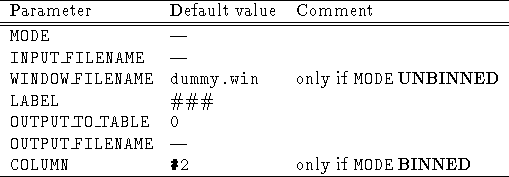
where: parfil is the name of the parameter file (created using the EXSAS command CREATE/PARFIL KS). The parameter file entries are shown in Table 7.15.

  
Table 7.15: Parameter file entries for MAKE/KSTEST

The meaning of the parameters is as follows:

• MODE is the accumulation mode. It can be:
  • BINNED: the input data are in BDT format. In this case no windowing is allowed. If a window file is specified, it will be read in, but it will not be used.
  • UNBINNED: the input data are in PET format.
• INPUT_FILENAME is the input table name. Default extension is TBL. There is no default.
• WINDOW_FILENAME is the name of the ASCII file containing the start-end times of the periods accepted for the analysis. It is always read in, but it is used only if the option UNBINNED is selected. The default filename for the window file is dummy.win. If the window file is not found, all times will be accepted. The default extension for window files is WIN.
• LABEL label for the output. This string will be written to the output table in the descriptor KS_COMMENT.
• OUTPUT_TO_TABLE is the flag for the production of an output table. If it is set to 1, the output table is produce; if it is 0, no output table will be produced.
• OUTPUT_FILENAME is the name of the (optional) output table containing the expected and observed distributions (and their difference. The default extension is TBL.
• COLUMN is the column identifier (either in the format #number or :label) for the column to which the analysis has to be applied. This allows the user to select, for instance, corrected light curves. It is read in only in the BINNED case, and in this case the default is '#2' (second column).
• Format of the output: the (optional) file in output from this command is:
  • K-S DISTRIBUTION: it is in the format of a MIDAS table with 4 columns. The first column contains the arrival times of the selected photons (with gaps removed) for the UNBINNED case, and the bin times for the BINNED case. The second column contains the expected distribution (which is a straight line going from 0.0 at the first photon/bin to 1.0 at the last). The third column is the observed distribution (also going from 0.0 to 1.0 by definition), and the fourth column is the absolute value of the difference between observed and expected. The descriptors of the main EXSAS header are copied from the first input table to the output power spectrum. Some new descriptors are created: the descriptor WINDOW_NAME (C*80) contains the window file name and the descriptor KS_COMMENT (C*80) contains the LABEL parameter read in from the parameter file. Besides, there are three more R*8 descriptors, named SIG_90, SIG_95 and SIG_99, which contain the 90%, 95% and 99% confidence levels for variability respectively. This values have to be compared to the R*8 descriptor KS_TEST giving the result of the K-S test. The output table can be used as input to the command PLOT/KSTEST.
  • LOGFILE: it is an ASCII file containing a copy of the output to terminal. The useful parameters read in from the parameter file are reported. The status of the window file opening and reading is displayed. The number of accepted photons (taking into account the user's window) is displayed. The output K-S test value and the 90%, 95% and 99% confidence limits for variability are then displayed. The logfile has the standard name kstest.log