Segmented Power Spectrum

 

The command MAKE/POWER_SPECTRUM produces in the option SEGMENTED a power spectrum   from data contained either in a list of BDTs or in a single PET. The input data are divided in stretches (maximum length 8192) and a power spectrum for a single stretch is produced. The output power spectrum (segmented power spectrum) is the average (frequency by frequency) of the single ones. The single power spectra are produced via Fast Fourier Transform   and they are normalized according to [Leahy et al.1983] In the BDT case the input tables do not have to be necessarily contiguous, but the same bin size is required. Any detected gap (which definition is specified by the user in a parameter) in the data will close the current data stretch and a new one will be started. If one of the input tables is not found, the program is closed at that time. All the parameters for the analysis (filenames included) are passed via a parameter file.

Different options are available: you can rebin your light curve before the power spectrum is performed (only in the BDT case), select special time intervals to be taken into account (windowing), choose the length for a single data stretch and apply a compression to the output power spectrum (either linear or logarithmic). In the PET case a value for the requested bin size is required, and it is possible to specify the starting time for the analysis, since in this case no window file will be used (data must be contiguous). It is also possible to produce a -T image,   in which all the single power spectra as a function of time are reported. The image is in a compressed format not suitable for immediate display. Use the command PREPARE/POWER_IMAGE to convert it into a good format for display. A parameter is available to select the minimum percentage exposure allowed to accept a bin; it is also possible to compute the power spectrum on the percentage exposure only (window function).

The syntax of the command is:

MAKE/POWER_SPECTRUM parfil S

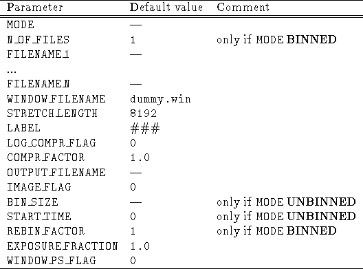
where parfil is the name of the parameter file, generated via CREATE/PARFIL SPOWER. The parameter file entries are shown in Table 7.11. The meaning of the parameters listed in Table 7.11 as follows:

  
Table 7.11: Parameter file entries for MAKE/POWER S

• MODE is the accumulation mode. It can be:
  • BINNED: the input data are in BDT format. Up to 9 different tables can be in input.
  • UNBINNED: the input data are in PET format. Only 1 table can be in input.
• N_OF_FILES is the number of input tables to be read in for the analysis in the BINNED case. The maximum number allowed is 9. Default is 1. In the UNBINNED case this parameter is unnecessary, because only one table can be in input.
• FILENAME_n is the n-th input table name. Default extension is TBL. There is no default.
• WINDOW_FILENAME is the name of the ASCII file containing the start-end times of the periods accepted for the analysis. The default filename for the window file is dummy.win. If the window file is not found, all times will be accepted. The default extension for window files is WIN.
• STRETCH_LENGTH is the length (in bins) of the single time stretch for the power spectrum evaluation. It must be a power of 2. The maximum value allowed (as well as the default) is 8192 ( ).
• LABEL label for the output. This string will be written to the output table (and optional image) in the descriptor POWER_COMMENT.
• LOG_COMPR_FLAG parameter for the logarithmic rebinning of power spectra. If this parameter is set to 0 the output spectrum is linearly rebinned, if it is 1 a logarithmic rebinning will be applied. Default value is 0.
• COMPR_FACTOR compression factor for the output power spectrum. If the parameter LOG_COMPR_FLAG is set to 0 the integer part of this parameter is taken as the linear rebinning factor for the power spectrum. If LOG_COMPR_FLAG is 0, this parameter is the logarithmic rebinning factor p, i.e. each bin will be a factor of  less than the preceding one. Default value is 1.
• OUTPUT_FILENAME is the filename of the output table containing the averaged power spectrum and of the optional -T image. The default extensions are TBL and BDF respectively.
• IMAGE_FLAG is the flag for the production of the -T image. If this parameter is set to 1 a -T image will be produced. Default value is 0.
• BIN_SIZE is the bin size for the light curve accumulation. It is required only in the UNBINNED case. There is no default.
• START_TIME it is the start time for the time series to be accepted for he analysis. If this value is used only if no window file is specified. The default value is 0.0. The default value is 0.
• REBIN_FACTOR is the rebin factor for the input data, used only in the BINNED case. By means of this parameter it is possible to rebin the data before the analysis. Default value is 1 (no rebinning). The rebinning is done internally and does not affect the data in the input BDTs.
• EXPOSURE_FRACTION is the minimum exposure fraction allowed for a bin to be selected as a ``good'' bin. If this parameter is set to 1.0 (the default) only fully exposed bins will be accepted. If it is set to 0.0 even complete gaps will be accepted as empty bins. All the intermediate values are of course allowed.
• WINDOW_PS_FLAG is the flag for the production of the power spectrum of the window function only. If it is set to 0 (the default), the normal power spectrum of the data will be computed. If it is set to 1, the power spectrum of the window function will be computed: this means that each selected bin will contain the percentage exposure of that bin rather than the detected counts. This option makes sense only if the parameter EXPOSURE_FRACTION is set to a value less than 1.0.
• Format of the input: the files input to this command are:
  • PARAMETER FILE: standard ASCII file generated via CREATE/PARFIL using the option SPOWER.
  • DATA TABLE(S): they are either BDTs or PETs as produced by the EXSAS projection package. Their format is described in section 7.2.2.
  • WINDOW FILE: it is a standard ASCII file. Each line of the file contains the start and end time of an accepted time interval. No comment lines are allowed.
• Format of the output: the files in output from this command are:
  • POWER SPECTRUM: it is in the format of a MIDAS table with 5 columns: frequency, error on frequency, power, error on power and significance respectively. The significance is the number of sigma of the power in a given bin above the white noise level, that is:

    

    where  is the power in the bin corresponding to the frequency  and  is the corresponding error. It can be plotted by using the MIDAS command PLOT/HISTO. In the BINNED case the descriptors of the main EXSAS header are copied from the first input table to the output power spectrum. Some new descriptors are created: the descriptor FFT_NUMBER (I*4) contains the total number of power spectra averaged, the descriptor WINDOW_NAME (C*80) contains the window file name and the descriptor POWER_COMMENT (C*80) contains the LABEL parameter read in from the parameter file.

  • -T image: it is in the format of a MIDAS bulk data frame. Frequency is running along the X-coordinate and time along the Y-coordinate. In addition the first column ([@1,@2:@1,>]) contains the count rate as a function of time, the second column ([@2,@2:@2,>]) contains the corresponding time, and the first row ([@3,@1:>,@1]) contains the frequency value. The elements [@1,@1] and [@2,@1] are left empty. The remaining sub-matrix [@3,@2:>,>] contains the values of the power for a given frequency and time. The handling of such an image (for either display or plot) is performed by other EXSAS commands (with qualifier POWER_IMAGE). The sub-matrix can be extracted for subsequent analysis by means of the MIDAS command EXTRACT/IMAGE new_image = image[@3,@2:>,>]. The same new descriptors as the output table (see above) are created.
  • LOGFILE: it is an ASCII file containing a copy of the output to terminal. The useful parameters read in from the parameter file are reported. The status of the window file opening and reading is displayed. For each single power spectrum is displayed a line containing: the index number of the power spectrum, the average count rate and the power in the first two bins (lower frequencies) of the power spectrum. Any data file opening is reported. The logfile has the standard name ps_seg.log