


Next: Hierarchical Wiener filtering
Up: Noise reduction from the
Previous: The convolution from the
The Wiener-like filtering in the wavelet space
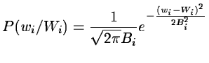
Let us consider a measured wavelet coefficient wi at the scale i.
We assume
that its value, at a given scale and a given position,
results from a noisy process, with a Gaussian distribution with a
mathematical expectation Wi, and a standard deviation Bi:
 |
|
|
(14.76) |
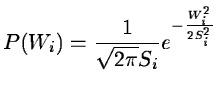
Now, we assume that the set of expected coefficients Wi for a given
scale also follows a Gaussian distribution, with a null mean and a
standard deviation Si:
 |
|
|
(14.77) |
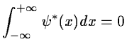
The null mean value results from the wavelet property:
 |
|
|
(14.78) |
We want to get an estimate of Wi knowing wi. Bayes' theorem gives:
 |
|
|
(14.79) |
We get:
 |
|
|
(14.80) |
where:
 |
|
|
(14.81) |
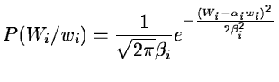
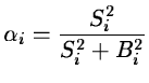
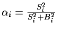
the probability
P(Wi/wi) follows a Gaussian distribution with a mean:
 |
|
|
(14.82) |
and a variance:
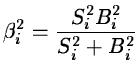 |
|
|
(14.83) |
The mathematical expectation of Wi is
 .
.
With a simple multiplication of the coefficients by the constant  ,
we get a linear filter. The algorithm is:
,
we get a linear filter. The algorithm is:
- 1.
- Compute the wavelet transform of the data. We get wi.
- 2.
- Estimate the standard deviation of the noise B0 of the first plane
from the histogram of w0. As we process oversampled images, the
values of the wavelet image corresponding to the first scale (w0)
are due mainly to the noise. The histogram shows a Gaussian peak
around 0. We compute the standard deviation of this Gaussian
function, with a
 clipping, rejecting pixels where the signal
could be significant;
clipping, rejecting pixels where the signal
could be significant;
- 3.
- Set i to 0.
- 4.
- Estimate the standard deviation of the noise Bi from B0. This
is done from the study of the variation of the noise between two
scales, with an hypothesis of a white gaussian noise;
- 5.
-
Si2 = si2 - Bi2 where si2 is the variance of wi.
- 6.
-
 .
.
- 7.
-
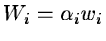 .
.
- 8.
- i = i + 1 and go to 4.
- 9.
- Reconstruct the picture from Wi.
Next: Hierarchical Wiener filtering
Up: Noise reduction from the
Previous: The convolution from the
Petra Nass
1999-06-15