In the following we ignore the pre-flash and skim term, and hence only take the bias and dark frames into account. The objective in reducing CCD frames is to determine the relative intensity Iij of a science data frame. In order to do this, at least two more frames are required in addition to the science frame, namely:
The dark current dark is measured in absence of any external input signal.
By considering a number of dark exposures a medium <dark> can be
determined:
The method to correct the frame for multiplicative spatial systematics is
know as flat fielding. Flat fields are made by illuminating the CCD with
a uniformly emitting source. The flat field then describes the sensitivity
over the CCD which is not uniform. A mean flat field frame with a higher
S/N ratio can be obtained buy combining a number of flat exposures. The
mean flat field and the science frame can be described by:
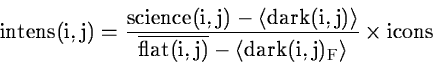
Combining Eqs.(3.2), (3.3) and (3.4) we isolate:
Here icons can be any number, and term
![]() now
denotes a dark frame obtained by e.g. applying a local median over a
stack of single dark frames. The subscript in
now
denotes a dark frame obtained by e.g. applying a local median over a
stack of single dark frames. The subscript in
![]() denotes that this dark exposures may necessarily be the same frame
used to subtract the additive spatial systematics from the raw science frame.
denotes that this dark exposures may necessarily be the same frame
used to subtract the additive spatial systematics from the raw science frame.
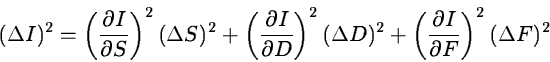
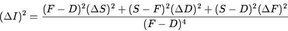
The mean absolute error of
intens(i,j) yields with icons = 1 (only the
first letter is used for abbreviations):
A small error ![]() is obtained if
is obtained if ![]() ,
,
![]() and
and
![]() are kept small. This is achieved by averaging Dark, Flat and
Science frames.
are kept small. This is achieved by averaging Dark, Flat and
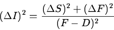
Science frames. ![]() is further reduced if S=F, then
Equation (3.8) simplifies to
is further reduced if S=F, then
Equation (3.8) simplifies to
This equation holds only at levels near the sky-background and is relevant for detection of low-brightness emission. In practice however it is difficult to get a similar exposure level for the flatfrm and science since the flats are usually measured inside the dome. From this point of view it is desirable to measure the empty sky (adjacent to the object) just before or after the object observations. In the case of infrared observations this is certainly advisable because of variations of the sky on short time scales.