The first filtering is then performed by a twice magnified scale
leading to the
![]() set. The signal difference
set. The signal difference
![]() contains the information between these two scales and is
the discrete set associated with the wavelet transform corresponding
to
contains the information between these two scales and is
the discrete set associated with the wavelet transform corresponding
to ![]() .
The associated wavelet is therefore
.
The associated wavelet is therefore ![]() .
.
 |
(14.29) |
The distance between samples increasing by a factor 2 from the scale (i-1) (i > 0) to the next one, ci(k) is given by:
 |
(14.30) |
and the discrete wavelet transform wi(k) by:
| wi(k) = ci-1(k) - ci(k) | (14.31) |
The coefficients ![]() derive from the scaling function
derive from the scaling function ![]() :
:
 |
(14.32) |
The algorithm allowing one to rebuild the data frame is evident: the
last smoothed array cnp is added to all the differences wi.
If we choose the linear interpolation for the scaling function ![]() (see figure 14.5):
(see figure 14.5):
![\begin{displaymath}\begin{array}{ll}
\phi(x) = 1 - \mid x \mid & \mbox{ if } x \...
...,1] \\
\phi(x) = 0 & \mbox{ if } x \not \in [-1,1]
\end{array}\end{displaymath}](img660.gif)
 |
(14.34) |
c1 is obtained by:
 |
(14.35) |
 |
(14.36) |
The figure 14.6 shows the wavelet associated to the scaling function.
The wavelet coefficients at the scale j are:
 |
(14.37) |
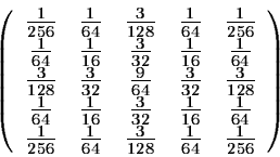
The above à trous algorithm is easily extensible to the two
dimensional space. This leads to a convolution with a mask of
![]() pixels for the wavelet connected to linear interpolation. The coefficents
of the mask are:
pixels for the wavelet connected to linear interpolation. The coefficents
of the mask are:

At each scale j, we obtain a set
![]() (we will call it
wavelet plane in the following), which has the same number of pixels
as the image.
(we will call it
wavelet plane in the following), which has the same number of pixels
as the image.
If we choose a B3-spline for the scaling function, the coefficients
of the convolution mask in one dimension are
(
![]() ), and
in two dimensions:
), and
in two dimensions:
