 |
First, there is a set of residual plots against airmass for each night. The plots for individual passbands are compressed so that two will fit on the screen at once; this allows you to notice correlations in the behavior of residuals in adjacent bands.
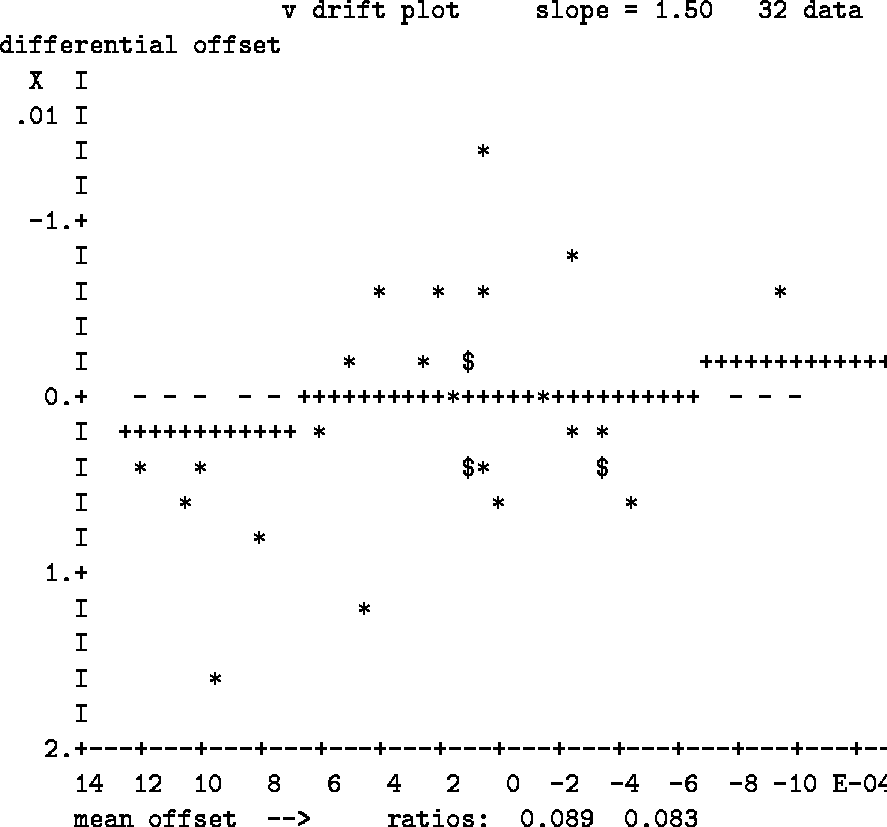
Next, there are residuals as functions of time for each night (again compressed to make comparisons easy). Examine these plots carefully for evidence of trends with time. After you have inspected the run of the residuals with time, the program will ask if you want to solve for time-dependent parameters. If you reply ``YES'', it will show you some plots intended to help you distinguish between time-dependent extinction and time-dependent zero-point drift. These plots are accompanied by some numbers that may also be helpful (see Fig. 13.3).
The principle behind these plots is that time-dependent extinction produces
errors (and hence, we hope, residuals) that are proportional to airmass;
but instrumental drift produces residuals uncorrelated with airmass.
Suppose we have two successive observations at airmasses M1 and M2,
which produce residuals
![]() and
and
![]() .
If the extinction changes slowly with time, we expect the ratios
.
If the extinction changes slowly with time, we expect the ratios
![]() and
and
![]() to be equal, as each is (on the average) the deviation of the current
extinction coefficient from the mean extinction for the night, multiplied by
the airmass difference of the points being compared.
to be equal, as each is (on the average) the deviation of the current
extinction coefficient from the mean extinction for the night, multiplied by
the airmass difference of the points being compared.
Unfortunately, a plot of the first ratio against the second produces an
uninformative scatter diagram, because the divisor
(M1 - M2 )makes the scatter of the points very unequal.
If, instead, we plot
![]() against
against
![]() ,
the values should all have comparable scatter.
This is the plot shown in Fig. 13.3.
The line drawn with + signs has the fitted slope and passes through the
origin.
Again, we expect unit slope if the extinction is changing with time,
and zero slope if the instrument is at fault.
The actual slope is printed above the plot.
,
the values should all have comparable scatter.
This is the plot shown in Fig. 13.3.
The line drawn with + signs has the fitted slope and passes through the
origin.
Again, we expect unit slope if the extinction is changing with time,
and zero slope if the instrument is at fault.
The actual slope is printed above the plot.
We can obtain additional information from the scatter of the values. The vertical spread of the plotted points is just proportional to a typical residual. The horizontal spread has the same value, but diminished by a typical value of the ratio (M1 - M2) / (M1 + M2 ). This average ratio, followed by the ratio of the spreads, is shown at the bottom of the plot. If the errors are dominated by changes in the extinction, we expect the ratio of spreads to be just this average ratio. But if instrumental drift dominates the errors, the spread in the ordinates should be much smaller than the spread in the abscissas, because the correlated part of the residuals cancels out in the differences.
If the drifts are small, so that the data are dominated by random noise, we expect the mean slope to be zero, and the ratio of spreads to be the average ratio of airmass difference to airmass sum, (M1 - M2) / (M1 + M2 ). We can therefore take a mean slope greater than 0.5 as evidence in favor of extinction drift, but a smaller slope is only weak evidence of zero drift, as it could be due to noise. Similarly, a spread ratio near zero is strong evidence for zero-point drift, but a value near the mean airmass ratio could be due to noise. On this basis, the sample data shown in Fig. 13.3 show good evidence for extinction drift.
After showing the individual drift plots, the program displays a table that summarizes the results for all bands and nights. In this table, cases that favor extinction drift are marked ``E'' and those that favor zero-point drift, ``Z''. Lower-case letters indicate weaker evidence, and a dash indicates nights with too few data to make a useful plot.
At this point, you will be asked to choose whether to solve for time-dependent extinction, time-dependent zero points, neither, or both. In general, you should choose the situation that seems most typical; help is available if you want it. It is usually not wise to try to solve for both kinds of drift; unless the data are very well distributed, one usually finds a strong anti-correlation of the derived drifts in extinction and zero-point. At present, only linear drifts with time are modelled; but this should suffice for most good nights.
If you choose to change the model (i.e., either add or remove a time-dependent term, compared to what was previously used), the program loops back to the beginning of the solution, and repeats its work, using the new model. Initially, solutions are always done without time-dependent terms. This strategy lets you choose an optimal set of extinction stars before trying to solve for any time-dependent terms, which are usually rather weakly determined. If you make no changes in the time-dependence of the model, the extinction solution is finished at this point.
If you included standard-star values in the extinction solution, the transformation coefficients were included in the parameter adjustments. Then full-screen plots of the transformation residuals are shown, followed by residuals plotted as a linearity check. If you did not include standard-star values, the linearity check is plotted, and the program then determines the transformation separately.