

Next: Statistical Tests
Up: Analysis of Results
Previous: Analysis of Results
The degree of correlation between two parameters can visually be
estimated by plotting them. Numerically this is expressed by the
correlation coefficient :
 |
(2.32) |
for the two variables x and y. This expression assumes that the
quantities have normal distribution. When the distribution is
unknown, the correlation can be given by the Spearman rank correlation
coefficient :
 |
(2.33) |
where n is the number of pairs and D is the difference of the rank
between x and y in a pair.
When the correlation coefficient indicates a significant correlation,
the functional relation is given by the regression line which is
computed by least squares methods for normal distributions or maximum
likelihood procedures (see Section 2.1.3). If non-linear
relations are expected, the variables are transformed into a linear
domain by means of standard mathematical functions. Such
transformation may also be used to make the variance of a variable
homogenous.
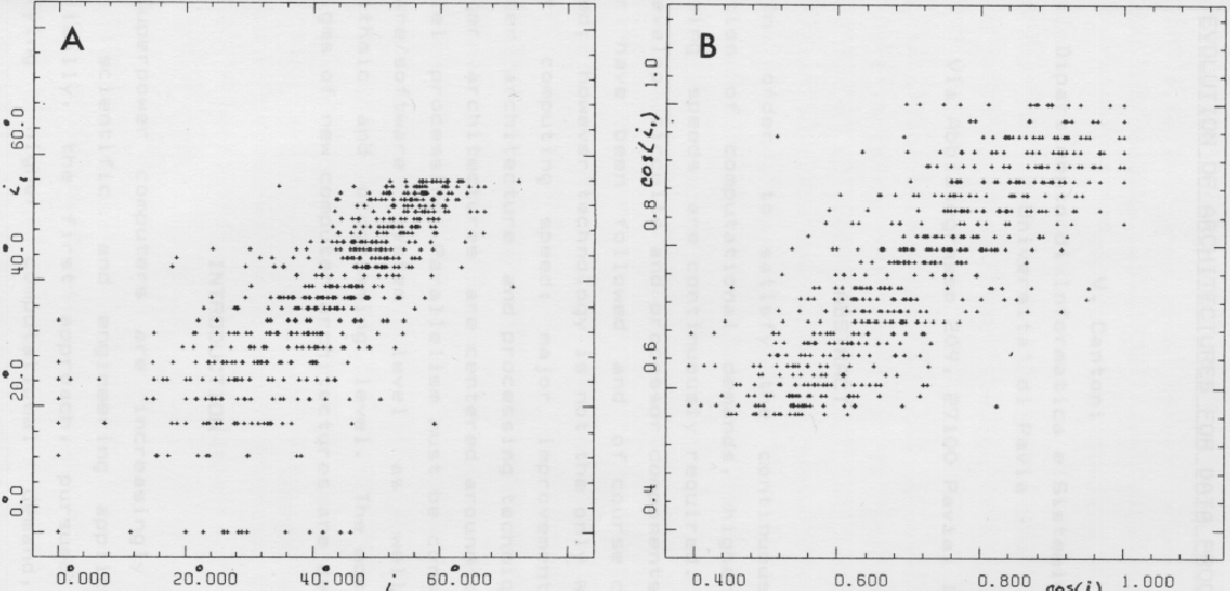
Figure 2.13:
Correlation between two measures of the inclination angle of
galaxies: (A) with angle i as variable, and (B) with
 .
.
 |
In Figure 2.13, a correlation between two different
measures of the inclination angle i of galaxies is shown. Since the
angle is obtained from the axial ratio, a cosine transformation is
used to achieve a homogenous variance. Unfortunately, it is not
always possible to obtain both a linear relation and homogeneity of
variance with the same transformation.
All methods assume that the single data points are unbiased and
uncorrelated. Great care must be taken to assure that this is
fulfilled. If this is not the case, significant systematic errors may
be introduced in the estimates. A standard example is magnitude
limited samples which may be affected by the Malmquist bias.


Next: Statistical Tests
Up: Analysis of Results
Previous: Analysis of Results
Petra Nass
1999-06-15

