

Next: Background Estimates
Up: Image Manipulations
Previous: Image Manipulations
The analog detector output is normally converted into integer values
so that the internal detector noise is resolved. This noise can be
reduced by replacing the pixels with an average of the surrounding
values using a linear filter. In general, the image I(m,n) is
convolved by a filter function F(i,j) giving the smooth image
 |
(2.16) |
In principle, the image S is smaller than the original because the
convolution is undefined along the edge. For convenience,
extrapolated values for F are used to avoid this reduction in size
after each filtering. Several different filter functions are used
depending on the application. Two typical
 filters are
given as examples, namely peaked smoothing filter
 |
(2.17) |
and a constant 'block' filter
 |
(2.18) |
Both filters are normalized to unity in order to preserve the total
flux in the image. Depending on the actual size and shape of the
filter, different degrees of smoothing are achieved (i.e. larger size
gives stronger smoothing). Filter functions which vary significantly
or are non-zero at the edge (e.g. Equation 2.18) will
tend to preserve some high frequencies in the output. The effects of
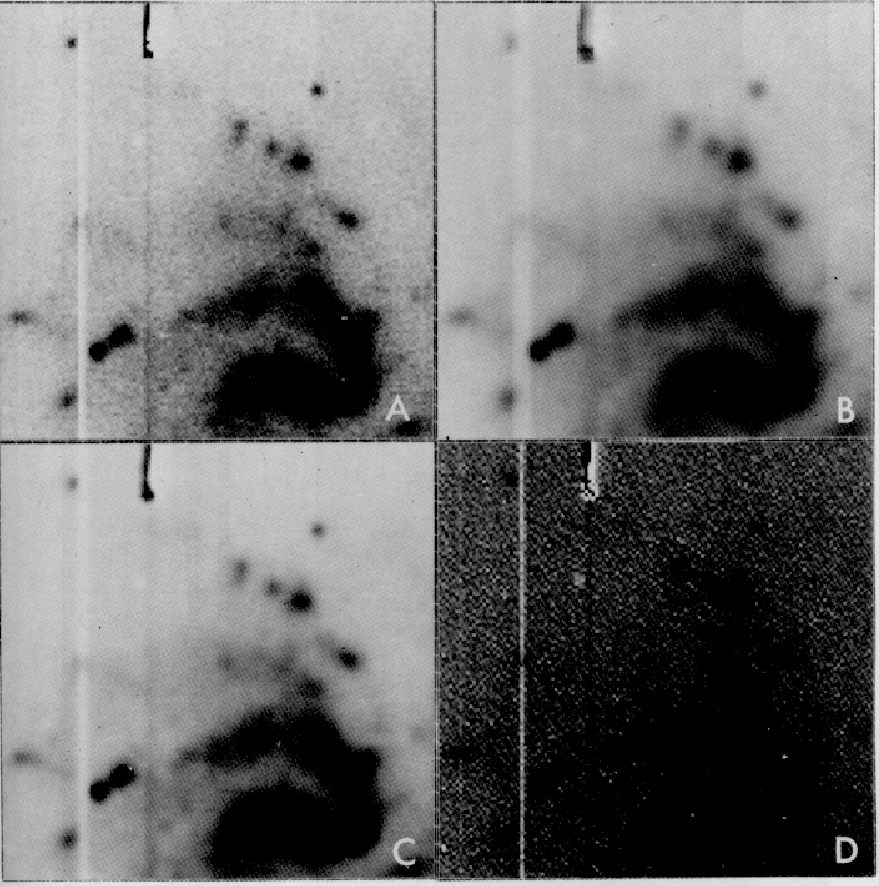
applying linear filters to a CCD frame is shown in
Figure 2.6.
Figure 2.6:
Different digital filters applied on a CCD image: (A) original,
(B) block filter, (C) smooth filter, and (D) Laplacian filter.
 |
It can be seen that the `block' filter leaves sharper features in the
result frame than the `smooth' filter. This is avoided by taking a
smooth function like a gaussian giving
![\begin{displaymath}F_{gaus} (j,k) = A \,
\exp \left( -\frac{1}{2} \left[ \frac{j^2}{\sigma_x^2} +
\frac{k^2}{\sigma_y^2} \right] \right)
\end{displaymath}](img74.gif) |
(2.19) |
where A is a normalization constant and  defines the width
of the filter. The parameters of the gaussian filter can normally be
varied to satisfy most applications (see Equation 2.19).
The increase in the S/N is paid by a degradation in the resolution.
When a fixed filter is used this blurring affects the whole frame;
although a smoothing may be required only in the low S/N regions.
This problem can be avoided by applying a gaussian filter for which
the width  is a function of the local S/N (e.g.
 ).
).
Other types of linear filters are used to emphasize edges and
variations. They are based on differential operators like the
Laplacian and have often
 to remove the mean level of
the input frame. A symmetric edge detection filter may be defined as
 |
(2.20) |
while a large variety of other filters may be constructed to enhance
special features. The result of the
FLaplace filter is shown in
Figure 2.6.
In some cases types of objects (e.g. stars) may disturb the further
analysis of an image. If these objects have a special appearance if
is often possible to remove them with a non-linear filter (see
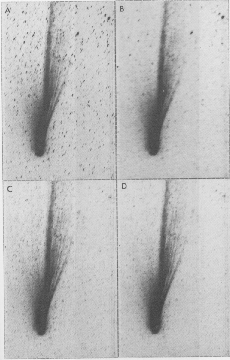
Section 2.2.1). To remove stellar images from a picture of
comet Halley, the results of applying different non-linear filters to
the frame are given in Figure 2.7. For more
complicated features they are deleted from the image by interpolation
between pixels in nearby regions.
Figure 2.7:
Removal of stars from a CCD frame of Comet Halley: (A) original,
(B)
 median filter, (C)
 recursive filter,
and (D) both recursive
 filter and a
 median filter.
 |


Next: Background Estimates
Up: Image Manipulations
Previous: Image Manipulations
Petra Nass
1999-06-15


![]() is a function of the local S/N (e.g.
is a function of the local S/N (e.g.
![]() ).
).
![]() to remove the mean level of
the input frame. A symmetric edge detection filter may be defined as
to remove the mean level of
the input frame. A symmetric edge detection filter may be defined as
