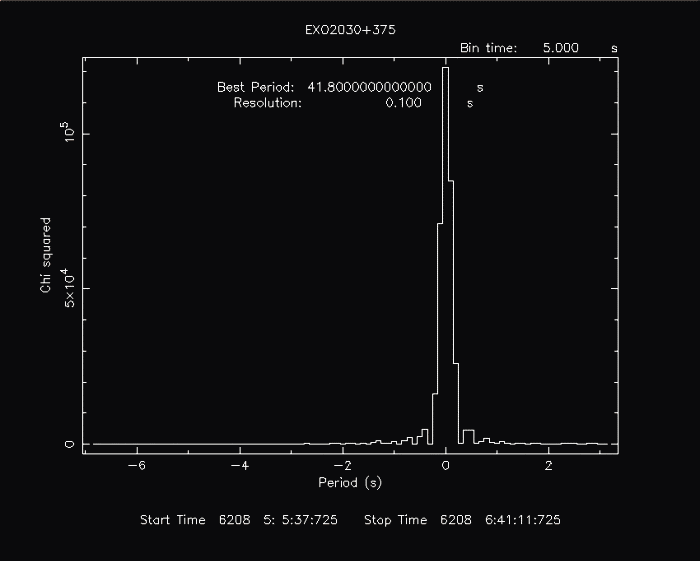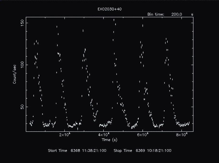
In this example, we plot the light curve of a single time series from EXOSAT ME of the transient pulsar, EXO 2030+375. The light curve data is made of multiple files listed in all.txt:
    d63924.lc.Z
    d63934.lc.Z
    d63945.lc.Z
    d63954.lc.Z
    d63968.lc.Z
    d63980.lc.Z
Executing the lcurve task:
    lcurve 1.0 (xronos5.18)

    Number of time series for this task[1]
    Ser. 1 filename +options (or @file of filenames +options)[file1] @all.txt
We enter the filelist beginning with an @ symbol, and lcurve reads in the files listed in all.txt
     Series 1 file   1:d63924.lc.Z

     Selected FITS extensions: 1 - RATE TABLE;

     Source ............ EXO2030+40          Start Time (d) ....  6368 11:36:56.100
     FITS Extension ....  1 - `RATE      `   Stop Time (d) .....  6368 14:28:08.127
     No. of Rows .......          342        Bin Time (s) ......    30.00
     Right Ascension ... 307.624755960       Internal time sys.. Converted to TJD
     Declination ....... 37.416656430        Experiment ........ EXOSAT   ME

     Corrections applied: Vignetting - Yes; Deadtime - Yes; Bkgd - Yes; Clock - No
                 values: .964785340       .911577050       1.00000000

     Selected Columns:  1- Y-axis;  2- Y-error;

     File contains binned data.

     Series 1 file   2:d63934.lc.Z

     Selected FITS extensions: 1 - RATE TABLE;

     Source ............ EXO2030+40          Start Time (d) ....  6368 14:44:12.129
     FITS Extension ....  1 - `RATE      `   Stop Time (d) .....  6368 18:24:28.162
     No. of Rows .......          440        Bin Time (s) ......    30.00
     Right Ascension ... 307.624755960       Internal time sys.. Converted to TJD
     Declination ....... 37.416656430        Experiment ........ EXOSAT   ME

     Corrections applied: Vignetting - Yes; Deadtime - Yes; Bkgd - Yes; Clock - No
                 values: .983090820       .909090880       1.00000000

     Selected Columns:  1- Y-axis;  2- Y-error;

     File contains binned data.

     Series 1 file   3:d63945.lc.Z

     Selected FITS extensions: 1 - RATE TABLE;

     Source ............ EXO2030+40          Start Time (d) ....  6368 18:38:52.164
     FITS Extension ....  1 - `RATE      `   Stop Time (d) .....  6368 21:16:44.185
     No. of Rows .......          315        Bin Time (s) ......    30.00
     Right Ascension ... 307.624755960       Internal time sys.. Converted to TJD
     Declination ....... 37.416656430        Experiment ........ EXOSAT   ME

     Corrections applied: Vignetting - Yes; Deadtime - Yes; Bkgd - Yes; Clock - No
                 values: .964785340       .910746750       1.00000000

     Selected Columns:  1- Y-axis;  2- Y-error;

     File contains binned data.

     Series 1 file   4:d63954.lc.Z

     Selected FITS extensions: 1 - RATE TABLE;

     Source ............ EXO2030+40          Start Time (d) ....  6368 21:32:12.186
     FITS Extension ....  1 - `RATE      `   Stop Time (d) .....  6369 01:48:04.208
     No. of Rows .......          511        Bin Time (s) ......    30.00
     Right Ascension ... 307.624755960       Internal time sys.. Converted to TJD
     Declination ....... 37.416656430        Experiment ........ EXOSAT   ME

     Corrections applied: Vignetting - Yes; Deadtime - Yes; Bkgd - Yes; Clock - No
                 values: .983090820       .909918130       1.00000000

     Selected Columns:  1- Y-axis;  2- Y-error;

     File contains binned data.

     Series 1 file   5:d63968.lc.Z

     Selected FITS extensions: 1 - RATE TABLE;

     Source ............ EXO2030+40          Start Time (d) ....  6369 02:05:24.209
     FITS Extension ....  1 - `RATE      `   Stop Time (d) .....  6369 05:47:16.215
     No. of Rows .......          443        Bin Time (s) ......    30.00
     Right Ascension ... 307.624755960       Internal time sys.. Converted to TJD
     Declination ....... 37.416656430        Experiment ........ EXOSAT   ME

     Corrections applied: Vignetting - Yes; Deadtime - Yes; Bkgd - Yes; Clock - No
                 values: .945537030       .911577050       1.00000000

     Selected Columns:  1- Y-axis;  2- Y-error;

     File contains binned data.

     Series 1 file   6:d63980.lc.Z

     Selected FITS extensions: 1 - RATE TABLE;

     Source ............ EXO2030+40          Start Time (d) ....  6369 06:03:00.215
     FITS Extension ....  1 - `RATE      `   Stop Time (d) .....  6369 10:18:36.212
     No. of Rows .......          510        Bin Time (s) ......    30.00
     Right Ascension ... 307.624755960       Internal time sys.. Converted to TJD
     Declination ....... 37.416656430        Experiment ........ EXOSAT   ME

     Corrections applied: Vignetting - Yes; Deadtime - Yes; Bkgd - Yes; Clock - No
                 values: .983090820       .909918130       1.00000000

     Selected Columns:  1- Y-axis;  2- Y-error;

     File contains binned data.

    Name of the window file ('-' for default window)[-]
Entering a - indicates that the default exposure
windows are to be applied ($XRDEFAULTS/default_win.wi). A custom
windows file may be generated with the xronwin task.
     Expected Start ...  6368.48398263830  (days)      11:36:56:100  (h:m:s:ms)
     Expected Stop ....  6369.42958578854  (days)      10:18:36:212  (h:m:s:ms)

     Minimum Newbin Time    30.000000      (s)
     for Maximum Newbin No..             2724

     Default Newbin Time is:   159.75775    (s) (to have 1 Intv. of     512 Newbins)
     Type INDEF to accept the default value

    Newbin Time or negative rebinning[4.6692607009327] 200
Entering INDEF would divide the total timespan of the data into 512 equal newbins. Note: the number 512 may be modified with the hidden parameter, nbdf. You may not enter a newbin value less than the Minimum Newbin Time, which corresponds to the largest bin size found in the input files. In this example, we choose a newbin time of 200.
     Newbin Time ......     200.00000      (s)
     Maximum Newbin No.               409

     Default Newbins per Interval are:         409
     (giving       1 Interval of          409 Newbins)
     Type INDEF to accept the default value

    Number of Newbins/Interval[10] indef
Entering INDEF includes the whole timespan of the input in the resulting plot. In order to subdivide the time series into multiple intervals, resulting in multiple plots, give a smaller number than the indicated INDEF value.
     Maximum of       1 Intvs. with          409 Newbins of       200.000     (s)
    Name of output file[default]
In this example, we enter a space before pressing Return to indicate that an output FITS file is not desired, however, entering default for the output file, will result in a binned FITS light curve file to be written with the extension .flc. Note: In cases using a filelist, entering a specific filename rather than default is recommended, as the default output file uses only the first file in the list to construct the file name.
Do you want to plot your results?[yes]
In general, we want to plot the binned light curve, however, entering no will prevent lcurve from plotting the output. This is useful when only the output FITS file is desired.
Enter PGPLOT device[/XW]
The Xwindows device, /xw is recommended as the results may be viewed immediately and the plot may be manipulated interactively with PLT. In some cases, however, other file-based devices such as /ps and /gif may be desired.
         409 analysis results per interval


     Intv    1   Start  6368 11:38:21
         Ser.1     Avg  53.04        Chisq 0.6966E+06   Var  1026.     Newbs.    390
                   Min  23.93          Max  153.7    expVar 0.5855      Bins   2559
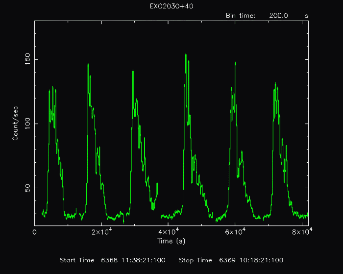
At this point the default lcurve plot is produced.

It may, however, by manipulated with any PLT command.
PLT> line step
Connect the points.
PLT> color 3 on 2
Change group 2 (the data representing Y) to color 3 (green).
PLT> r x 0 82000
Rescale the x-axis from 0 to 82000.
PLT> r y,,180
Rescale the y-axis from the current minimum value to 180.
PLT> cpd exo2030_375.gif/gif
Change the plot device to a gif.
PLT> p
Plot to the gif.
PLT> quit
See the modified lcurve plot for the effects of the commands.
Note: If a particular sequence of commands is to be used multiple times, using a plot file may save some time. Rather than entering PLT commands interactively, a script file containing the commands usually with the extension .pco can be given for the hidden parameter, plotfile. For example, we can place the interactive commands used above into the file lcurve.pco:
    line step
    color 3 on 2
    r x 0 82000
    cpd exo2030_375.gif/gif
    p
    quit
If lcurve is executed like this:
> lcurve plotfile=lcurve.pco
The program will execute the commands, creating the exo2030_375.gif graphic and exiting the program automatically with no interaction at the PLT prompt. This is a useful option for automated plot generation provided all the required parameters are set when the task is executed.
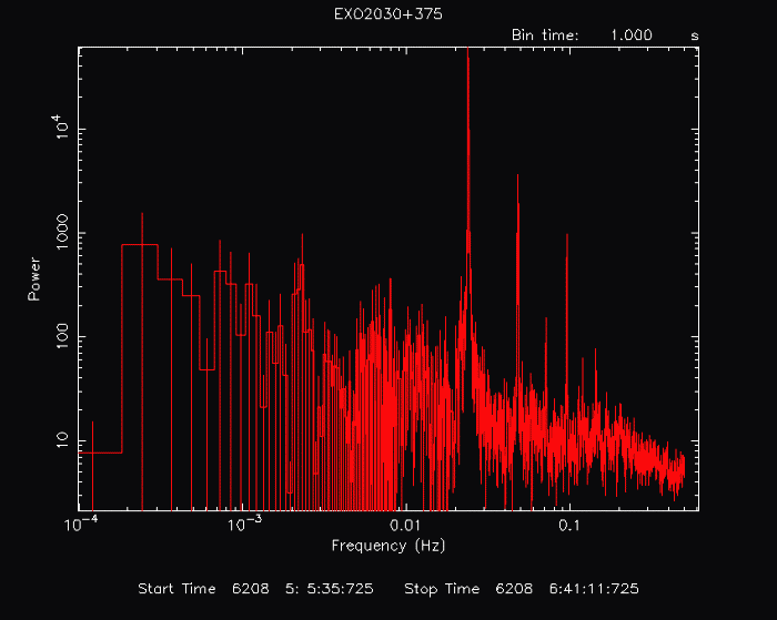
In this example, we plot the power spectrum of a time series from EXOSAT ME of the transient pulsar, EXO 2030+375.
Executing the powspec task:
    powspec 1.0 (xronos5.18)

    Ser. 1 filename +options (or @file of filenames +options)[file1] me_a52385.lc.Z
     Series 1 file   1:me_a52385.lc.Z
We enter a single filename here, however a list of files in the series may be given as a filelist beginning with an @ symbol if there are multiple files.
     Selected FITS extensions: 1 - RATE TABLE;

     Source ............ EXO2030+375         Start Time (d) ....  6208 05:05:35.725
     FITS Extension ....  1 - `RATE      `   Stop Time (d) .....  6208 06:41:19.250
     No. of Rows .......         5737        Bin Time (s) ......    1.000
     Right Ascension ... 307.588622760       Internal time sys.. Converted to TJD
     Declination ....... 37.382217390        Experiment ........ EXOSAT   ME

     Corrections applied: Vignetting - Yes; Deadtime - Yes; Bkgd - Yes; Clock - No
                 values: .983574270       .756429610       1.00000000

     Selected Columns:  1- Y-axis;  2- Y-error;

     File contains binned data.

    Name of the window file ('-' for default window)[-]
Entering a - indicates that the default exposure windows are to be applied ($XRDEFAULTS/default_win.wi). A custom windows file may be generated with the xronwin task.
     Expected Start ...  6208.21221903629  (days)       5: 5:35:725  (h:m:s:ms)
     Expected Stop ....  6208.27869502456  (days)       6:41:19:250  (h:m:s:ms)

     **** Warning: Newbin Time must be an integer multiple of Minimum Newbin Time
     Minimum Newbin Time    1.0000000      (s)
     for Maximum Newbin No..             5744

     Default Newbin Time is:   1.0000000    (s) (to have 1 Intv. of    8192 Newbins)
     Type INDEF to accept the default value

    Newbin Time or negative rebinning[4.6692607009327] 1
You may not enter a newbin value less than the Minimum Newbin Time, which corresponds to the largest bin size found in the input file. In this example, we choose a newbin time of 1, thus the original binning is preserved.
     Newbin Time ......     1.0000000      (s)
     Maximum Newbin No.              5744

     Default Newbins per Interval are:        8192
     (giving       1 Interval of         8192 Newbins)
     Type INDEF to accept the default value

    Number of Newbins/Interval[10] INDEF
Entering INDEF includes the whole timespan of the input in the resulting plot. In order to subdivide the time series into multiple intervals, resulting in multiple plots, give a smaller number than the indicated INDEF value.
     Maximum of       1 Intvs. with         8192 Newbins of       1.00000     (s)
    Default intervals per frame are:         1
    Type INDEF to accept the default value
    Number of Intervals/Frame[1]
If multiple intervals exist, frames may be calculated from the average of some of them and then plotted. One frame corresponds to one plot. In this example, we have only one interval, and consequently one frame and one plot.
     Results from up to       1 Intvs. will be averaged in a Frame
    Rebin results? (>1 const rebin, <-1 geom. rebin, 0 none)[0]
The first time through we will use no binning, setting the value to 0. The unbinned plot appears first at the end of the example. Then we will use a geometric rebinning, entering a value of -1.01, the results of which are represented in the second plot below. A rebin value less than -1 corresponds to binning as a geometrical series with a step equal to the modulus. In this example, the step is 0.01.
Name of output file[default]
In this example, we enter a space before pressing Return to indicate that an output FITS file is not desired, however, entering default for the output file, will result in a binned FITS light curve file to be written with the extension .fps.
Do you want to plot your results?[yes]
In general, we want to plot the power spectrum, however, entering no will prevent powspec from plotting the output. This is useful when only the output FITS file is desired.
Enter PGPLOT device[/XW]
The Xwindows device, /xw is recommended as the results may be viewed immediately and the plot may be manipulated interactively with PLT. In some cases, however, other file-based devices such as /ps and /gif may be desired.
        4096 analysis results per interval

     Intv    1   Start  6208  5: 5:35
         Ser.1     Avg  401.0        Chisq 0.1627E+06   Var 0.1594E+05 Newbs.   5713
                   Min  152.8          Max  826.5    expVar  559.6      Bins   5713
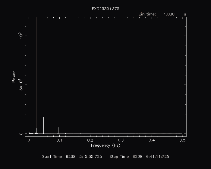
    Power spectrum ready !
At this point the default powspec plot (no rebinning) is produced.
Now, assume we run powspec again using the rebin value of -1.01, and then use the following PLT commands:
PLT> color 2 on 2
Change group 2 (the data representing Y) to color 2 (red).
PLT> cpd exo2030_375ps.gif/gif
Change the plot device to a gif.
PLT> p
Plot to the gif.
PLT> quit
See the modified powspec plot for the effects of the commands.
In this example, we search for the period of a light curve from EXOSAT ME of the transient pulsar, EXO 2030+375.
Executing the efsearch task:
    efsearch 1.1 (xronos5.18)

    Ser. 1 filename +options (or @file of filenames +options)[file1] me_a52385.lc.Z
     Series 1 file   1:me_a52385.lc.Z
We enter the light curve, me_a52385.lc.Z directly as the time series to be considered.
     Selected FITS extensions: 1 - RATE TABLE;

     Source ............ EXO2030+375         Start Time (d) ....  6208 05:05:35.725
     FITS Extension ....  1 - `RATE      `   Stop Time (d) .....  6208 06:41:19.250
     No. of Rows .......         5737        Bin Time (s) ......    1.000
     Right Ascension ... 307.588622760       Internal time sys.. Converted to TJD
     Declination ....... 37.382217390        Experiment ........ EXOSAT   ME

     Corrections applied: Vignetting - Yes; Deadtime - Yes; Bkgd - Yes; Clock - No
                 values: .983574270       .756429610       1.00000000

     Selected Columns:  1- Y-axis;  2- Y-error;

     File contains binned data.

    Name of the window file ('-' for default window)[-]
Entering a - indicates that the default exposure windows are to be applied ($XRDEFAULTS/default_win.wi). A custom windows file may be generated with the xronwin task.
     Expected Start ...  6208.21221903629  (days)       5: 5:35:725  (h:m:s:ms)
     Expected Stop ....  6208.27869502456  (days)       6:41:19:250  (h:m:s:ms)

     Default Epoch is:  6208.000000
    Type INDEF to accept the default value
     Epoch format is days.
    Epoch[34 234.23] 6208
In this example we choose 6208.0 as the Epoch. Entering INDEF would have the same result.
     Period format is seconds.
    Period[88.87] 40
Enter a guess for the period (default units are seconds) of the light curve. The period value will be used as the center of the range of trial values.
     Expected Cycles ..            143.59
     Default phase bins per period are:         8
     Type INDEF to accept the default value
    Phasebins/Period {value or neg. power of 2}[-3]
The phasebins/period (nphase) setting represents the
resolution of the trial folded light curves
(i.e. the number of bins that the range from phase of 0.0
to phase of 1.0 is divided into). If a negative value is given, the
phasebins/period is 2 to the power of the absolute value of that
number.
(e.g. nphase=-3 -![]() nphase=2^{abs(-3)}=8). The default (8),
corresponding to INDEF may
be altered with the hidden parameter nbdf.
nphase=2^{abs(-3)}=8). The default (8),
corresponding to INDEF may
be altered with the hidden parameter nbdf.
     Newbin Time ......     5.0000000      (s)
     Maximum Newbin No.              1149

     Default Newbins per Interval are:        1149
     (giving       1 Interval of         1149 Newbins)
     Type INDEF to accept the default value

    Number of Newbins/Interval[10] 1149
Entering INDEF would include exactly the timespan of the input in the resulting plot. Giving a smaller number than the indicated INDEF value would result in multiple intervals. In this example, we enter the default value, 1149, directly so only one interval is calculated.
     Maximum of       1 Intvs. with         1149 Newbins of       5.00000     (s)
     Default resolution is 0.1392515231
     Type INDEF to accept the default value
    Resolution for period search {value or neg. power of 2}[.03] 0.1
     Default number of periods is       128
     Type INDEF to accept the default value
    Number of periods to search[100]
The period, resolution of period search, and number of periods to search together define the range of periods to search. In this example, 100 periods are searched around 40 seconds in steps of 0.1 (i.e. 35.0, 35.1, 35.2, ... 44.7, 44.8, 44.9)
Name of output file[default]
In this example, we enter a space before pressing Return to indicate that an output FITS file is not desired, however, entering default for the output file, will result in a folded FITS light curve file to be written with the extension .fes.
Do you want to plot your results?[yes]
In general, we want to plot the results of the search, however, entering no will prevent efsearch from plotting the output. This is useful when only the output FITS file is desired.
Enter PGPLOT device[/XW]
The Xwindows device, /xw is recommended as the results may be viewed immediately and the plot may be manipulated interactively with PLT. In some cases, however, other file-based devices such as /ps and /gif may be desired.
         100 analysis results per interval


     Period :   41.80    dP/dt :  0.0000E+00
     Intv    1   Start  6208  5: 5:37
         Ser.1     Avg  400.0        Chisq 0.1214E+06   Var 0.1171E+05 Newbs.      8
                   Min  268.6          Max  554.2    expVar 0.7800      Bins   5713
At this point the default efsearch plot is produced. Note that the x axis represents the attempted periods offset by the best period found.
